PhysPlot GUI Walkthrough

PhysPlot is a graphical scientific plotting application designed for publication-ready 2D plotting. It supports data import, manual data entry, mathematical data manipulation, plotting, fitting, figure export, and text-format data export. It also supports vector and bitmap output formats such as PDF, PostScript, SVG, and EPS, along with text, CSV, and Excel data import.

See the project repository for full project context: PhysPlot on GitHub.

This walkthrough follows the main GUI workflow:

1. Main window overview

2. Importing data

3. Choosing axis roles

4. Generating and formatting a plot

5. Curve fitting and fit labels

6. Custom file-loader system

7. Custom mathematical function system

8. Exporting processed data

1. Main Window Overview

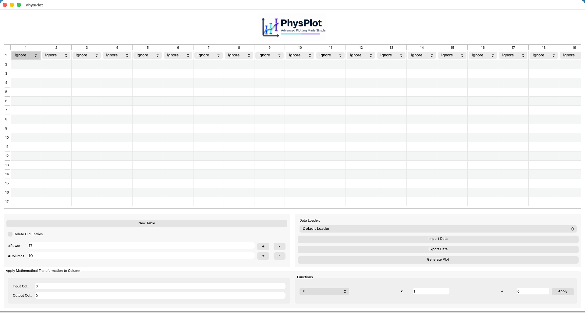
Figure 1. PhysPlot main window overview.

The PhysPlot main window provides a spreadsheet-style data table, column-role selectors, table controls, file import/export tools, plot generation controls, and mathematical transformation options in one interface.

When PhysPlot is launched, the main window opens with a spreadsheet-style table for entering or importing data. Each column has a dropdown menu at the top to assign the column role as X-axis, Y-axis, Xerr, Yerr, or Ignore.

The lower-left section contains table controls for creating a new table, deleting old entries, and changing row/column counts. The lower-right section contains the main data workflow controls, including Data Loader, Import Data, Export Data, and Generate Plot.

The bottom section provides transformation tools where users select an input column, define an output column, choose a function, set multiplier/offset values, and click Apply.

2. Importing Data

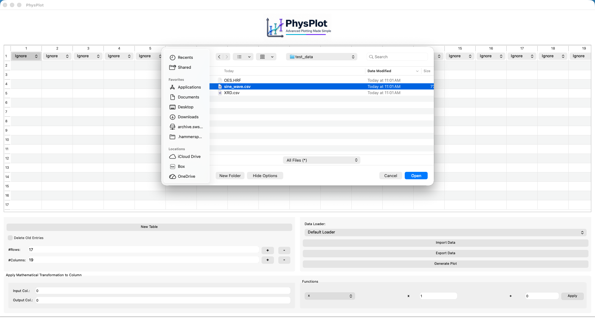
Figure 2. Selecting a data file for import.

To import data:

1. Select the required loader from Data Loader.

2. For standard tabular files, keep Default Loader selected.

3. Click Import Data.

4. Choose the data file in the file-selection dialog.

5. Click Open.

In this example, sine_wave.csv is selected from test_data. PhysPlot then loads the data into the table.

3. Choosing Axis Roles

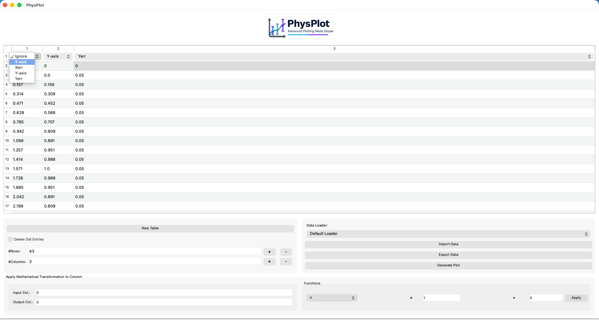
Figure 3. Choosing column roles for plotting.

After import, assign each column role from the dropdown in the top row. At minimum, set one X-axis column and one Y-axis column.

1. Open the dropdown above the independent-variable column.

2. Select X-axis.

3. Open the dropdown above the dependent-variable column.

4. Select Y-axis.

5. Optionally assign uncertainty columns as Xerr or Yerr.

6. Keep unused columns as Ignore.

4. Generating and Formatting a Plot

Figure 4. Generated plot with plot-formatting controls.

After assigning column roles, click Generate Plot. PhysPlot opens the plot window and the Configuration window. The Plot Formatting tab controls visual appearance.

Users can adjust grid style/width/color, marker style/size/color, and plot-line style/width. Click Apply after changes to update the active plot.

5. Curve Fitting and Fit Labels

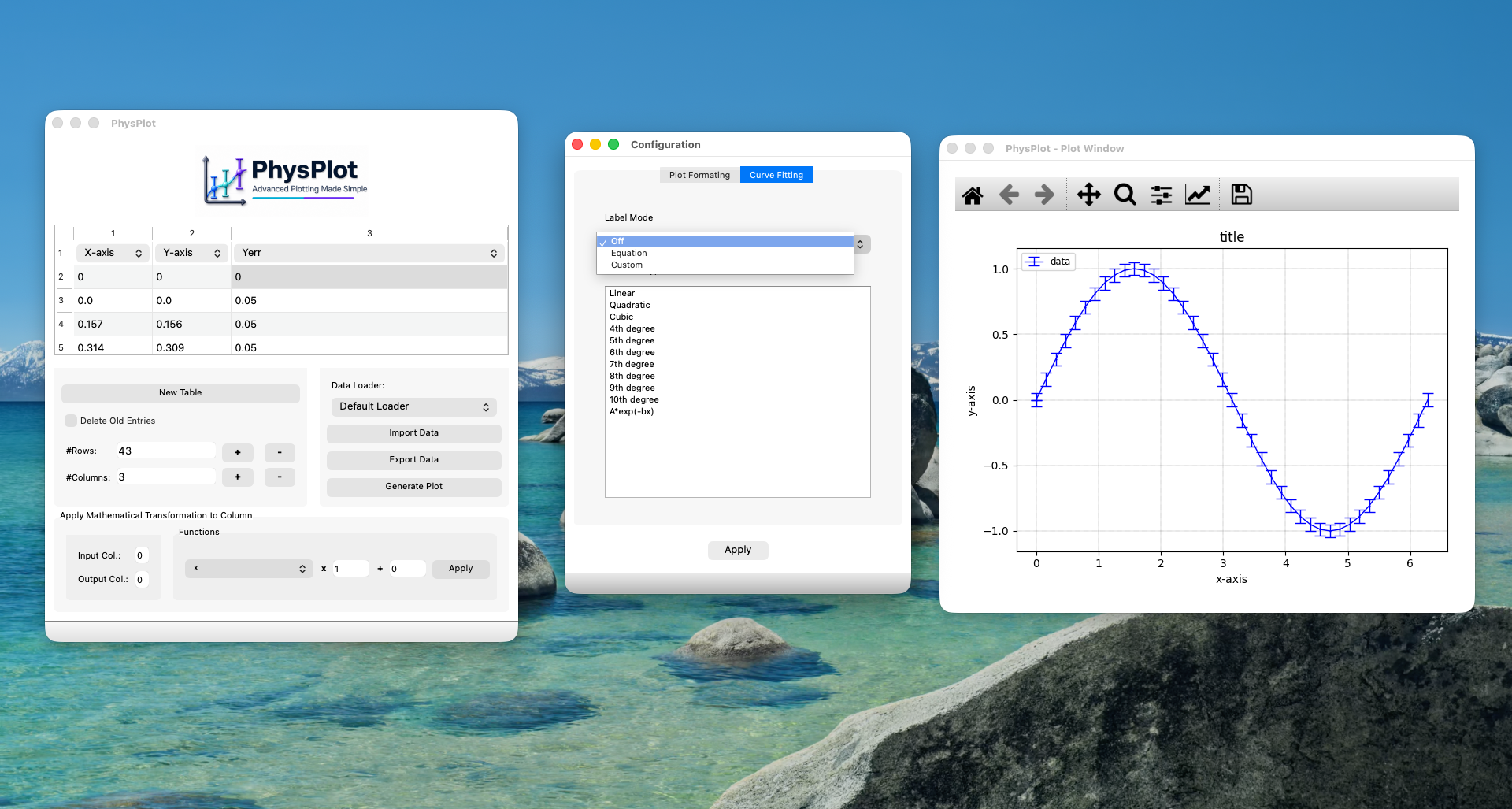
Figure 5. Curve fitting options and label mode selection.

Open Configuration -> Curve Fitting to apply fitting models such as linear, polynomial orders, and exponential models.

Label Mode controls fitting labels:

• Off: hide fit label.

• Equation: show fitted equation automatically.

• Custom: use a user-defined label.

Click Apply to update the plot.

6. Custom File-Loader System

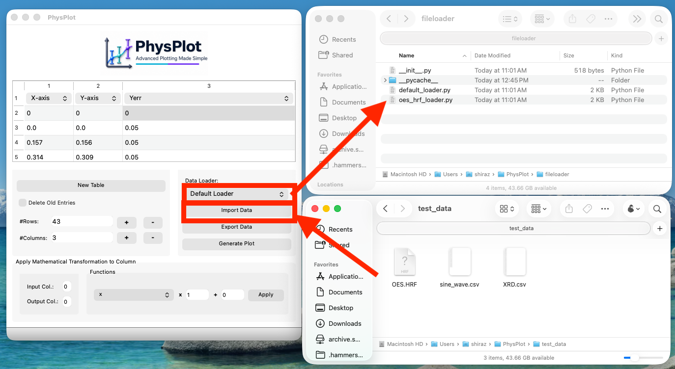
Figure 6. Custom file-loader system.

PhysPlot supports modular file loading via fileloader/. Each loader is a separate .py module for a specific file structure.

To use a custom loader:

1. Add/copy the loader module to fileloader/.

2. Restart PhysPlot if needed.

3. Select the loader from Data Loader.

4. Click Import Data.

5. Select the matching file.

7. Custom Mathematical Function System

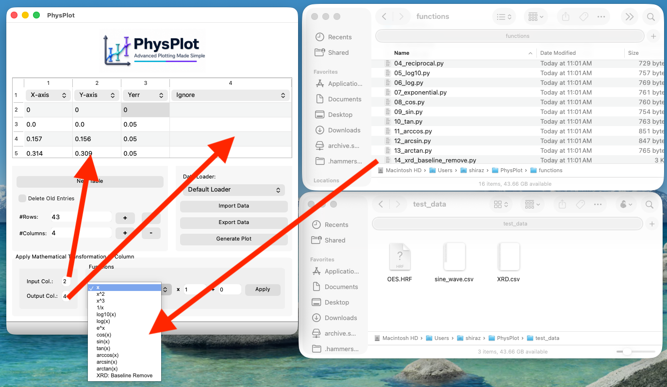
Figure 7. Custom mathematical transformation system.

PhysPlot applies mathematical transformations to selected columns.

General workflow:

1. Select Input Col..

2. Select Output Col..

3. Choose a function from Functions.

4. Optionally adjust multiplier and offset.

5. Click Apply.

6. The transformed data appear in the selected output column.

The Functions dropdown is generated from modules in functions/, making the system extensible for custom scientific workflows.

8. Exporting Processed Data

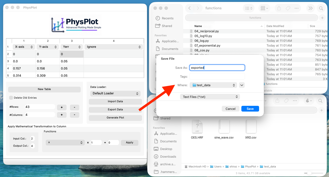
Figure 8. Exporting processed data.

To export current table data:

1. Click Export Data.

2. Choose destination folder.

3. Enter a filename.

4. Keep Text Files (*.txt).

5. Click Save.

This completes the core GUI workflow: import data, process data, plot data, customize and fit the plot, and export processed results.

Complete GUI Workflow Summary

1. Launch PhysPlot.

2. Enter data manually or import a data file.

3. Select the appropriate file loader if using a custom structure.

4. Assign column roles (X-axis, Y-axis, Xerr, Yerr).

5. Apply mathematical transformations if needed.

6. Generate the plot.

7. Customize plot formatting.

8. Apply curve fitting if required.

9. Choose fit-label mode (Off, Equation, or Custom).

10. Export processed data.

11. Save the final figure from the plot window toolbar.

Notes for Extending PhysPlot

PhysPlot v2.0.0 supports a modular extension workflow with these key locations:

• fileloader/ for custom file import structures

• functions/ for custom mathematical transformations

• curve-fitting configuration/modules for custom fitting behavior

This design helps users extend workflows for different instruments, data structures, and analysis routines without repeated edits to the main GUI.